Tutorials
Introduction
TRAPID is an online tool for the fast and efficient processing of assembled RNA-Seq transcriptome data. TRAPID offers high-throughput ORF detection, frameshift correction and includes a functional, comparative and phylogenetic toolbox. Input sequences can be ESTs, full-length cDNAs or RNA-Seq transcriptome sequences. Additionally, coding sequence derived from an annotated genome can also be used. We offer four reference databases: for plants and green algae, the latest PLAZA databases (PLAZA dicots and monocots 4.5, pico-PLAZA 3.0, PLAZA diatoms 1.0), and for other eukaryotes (e.g. Alveolata, Amoebozoa, Euglenozoa, Fungi, Metazoa) or prokaryotes (Bacteria and Archaea) eggNOG version 4.5 is available.
Once the initial processing has assigned functional annotations and gene families to the user-defined transcripts, evolutionary studies on gene families including the uploaded transcripts can be performed. Through a few simple operations, multiple sequence alignments and phylogenetic trees can be generated.
Although TRAPID hosts a wide range of reference genomes, it was not developed to process data from massive-scale meta -omic studies, as it can process 200,000 sequences maximum per experiment. Adding more transcripts is possible, but correct processing or website performance is not guaranteed in this case.
Account registration and login
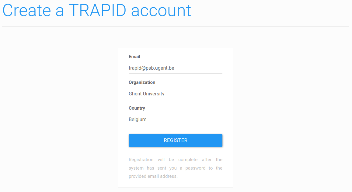
Figure 1: registration form. Fill in your information and click the 'register' button: an e-mail with login credentials will be sent.
Before you can use TRAPID, you need to register for an account. For academics, this is free of charge.
First, click on Register in the header (or click here).
On the next page, fill in the required information and click on the Register button (Figure 1). Make sure to provide a valid e-mail address as your login credentials will be sent immediately at this address.
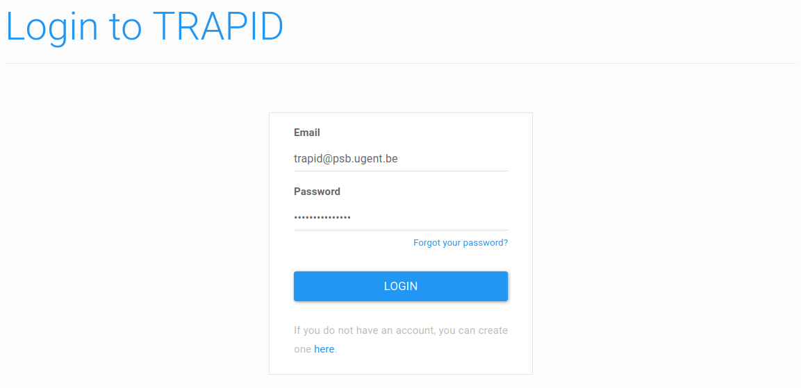
Figure 2: login form. Log in using your e-mail address and the provided password.
On the main page, click Login in the header (or click here).
This will take you to a login form (Figure 2). Here, use the e-mail address used to register and the password sent by mail to log in.
Tutorial 1: Panicum transcriptome functional annotation
In this tutorial, you'll learn how to functionally annotate and analyze the transcriptome of Panicum hallii (Meyer et al. 2012, Transcriptome analysis and gene expression atlas for Panicum hallii var. filipes, a diploid model for biofuel research.). The dataset can be obtained from the TRAPID FTP.
Part 1: uploading and processing the data
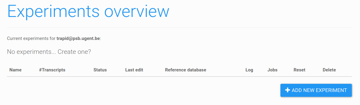
Figure 3: empty experiments overview. At the bottom of the page, click 'add new experiment' to create a new experiment.
After logging in, you will be redirected to the experiments overview. If you are a new user, this page will be empty (Figure 3). Please note this page can list two types of experiments:
- Current experiments (experiments you uploaded and own),
- Shared experiments (experiments uploaded by others you are allowed to view)
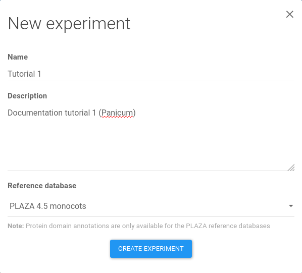
Figure 4: experiment creation. A name, a description, and reference database need to be chosen for the new experiment. Finalize the creation by clicking Create experiment.
Clicking on the add new experiment button ( icon) opens the experiment creation window (Figure 4).
To start, like shown in Figure 4, enter a name and a description for the experiment. For instance, Tutorial 1 as a name and Documentation tutorial 1 (Panicum) as description.
Select PLAZA 4.5 monocots as reference database, as PLAZA is the recommended database for plants and microbial photosynthetic eukaryotes, and the 'monocots' version contains genomes from closely related species.
In case data from other lineages is analyzed, we recommend selecting eggNOG 4.5. An overview of the available reference databases can be found on the
tools & parameters documentation page.
Add the experiment by clicking create experiment.
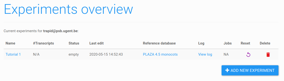
Figure 5: experiments overview. The newly created experiment appeared in the current experiments table. To add sequences, first click on the name of the experiment.
The new experiment will now appear in the current experiments table (Figure 5). Note that each user can create a maximum of 20 experiments.
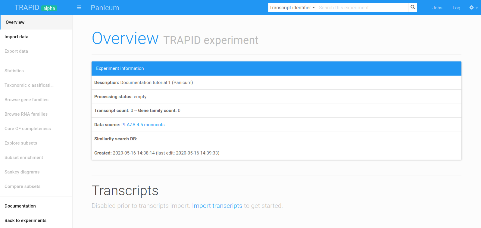
Figure 6: empty experiment overview page. The newly created experiment overview page. Click on Import data in the side menu to import sequences.
To continue, click on the experiment's name (e.g. Tutorial 1) in the current experiments table. This will take you to your newly created TRAPID experiment and display the experiment overview page (Figure 6). After transcripts sequences are processed, this page will contain general experiment statistics (in the Experiment information panel) and a detailed overview of the transcripts.
Two main elements may be used for navigating a TRAPID experiment: the experiment header (top) and the side menu (left). The experiment header contains links to experiment controls (jobs, log, and settings) and a search box to find specific sequences, gene/RNA families, or functional data. The side menu lists the main data import/export, exploration, and analysis options available within TRAPID. Note that in figure 6, all the items except Import data are disabled, since the experiment is empty.
To continue and upload input sequences, click on the Import data item of the side menu.
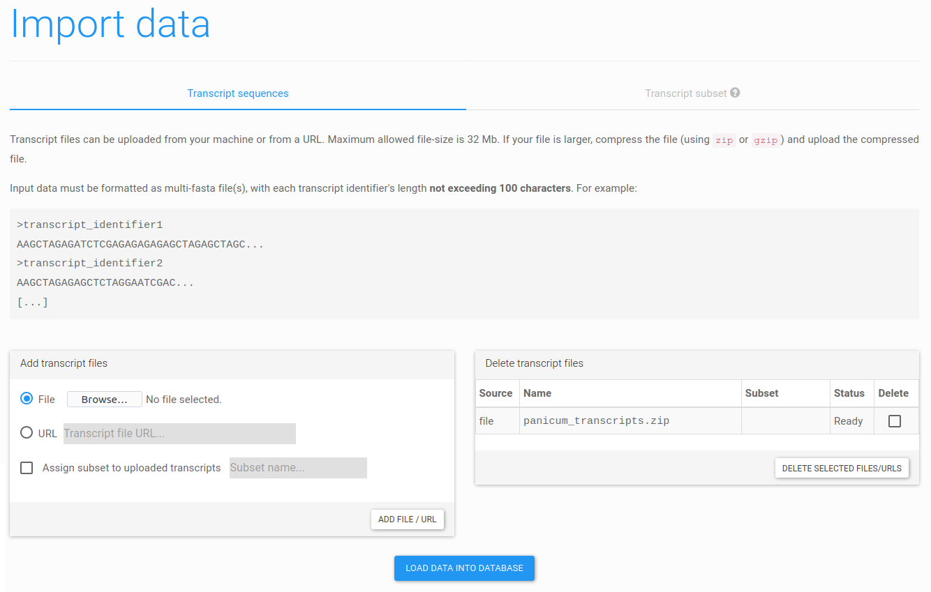
Figure 7: uploading transcript sequences. From this page, a dataset can be uploaded from a file or a URL. After adding files or URLs, please click Load data into database to upload the data.
Input sequences must be provided in FASTA format. Make sure each sequence has a unique identifier (max. 100 characters) and no empty sequences are present. Please note that individual files cannot be larger than 32Mb. For large datasets, we therefore recommend to supply compressed data (zipped or gzipped) and/or to split the data in multiple files.
In case you downloaded the tutorial dataset, you can upload the file (click Browse... and locate it on your system). Otherwise, you can directly supply the URL (https://ftp.psb.ugent.be/pub/trapid/datasets/panicum/panicum_transcripts.zip). After selecting a file or URL, click Add file/URL to confirm your choice and add the dataset. Afterwards, click Load data into database to load all sequences into our database. Both steps are essential before the data can be processed.
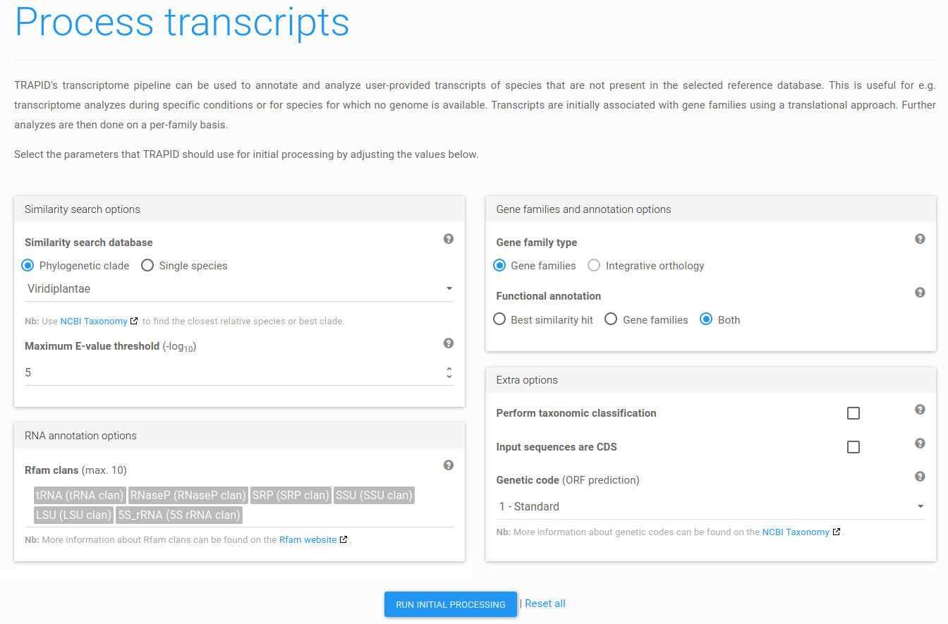
Figure 8: process transcripts. Select the desired settings for the various processing steps and click Run initial processing.
After the sequences have been loaded into the TRAPID database, the next step is to perform the initial processing. This step will add them to gene or RNA families, add annotations and a taxonomic label (if this step was enabled). To start the initial processing, go to your TRAPID experiment. Note how the page now contains a table with transcripts at the bottom, and how some options of the side menu have become enabled (although they only become useful after the processing). Click Process transcripts.
On the next page, you have to specify how transcripts should be processed by TRAPID. For this tutorial, select the settings as shown in Figure 8 (default settings except for the taxonomic classification that was disabled). More details on these settings can be found in the
general documentation.
Finish by clicking Run initial processing. Depending on the size of the dataset, the selected settings, and the load on our servers, this can take up to several hours. For this tutorial, it should take around one hour after starting. In the meantime, the experiment will be in processing state and cannot be accessed, except for the experiment's job management and log pages. An e-mail will be sent upon completion.
Once the initial processing has finished, all sequences will be included in gene/RNA families and be annotated (when possible). Additionally, as transcript data often includes truncated sequences or sequences with indels, potentially problematic sequences are flagged.
Part 2: exploring TRAPID output
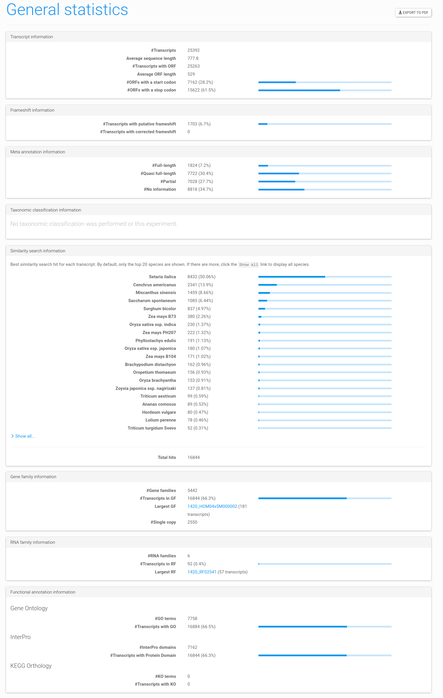
Figure 9: the general statistics page. This page displays general information that can be used to assess the quality of the transcripts, their taxonomic classification (if performed), how many were assigned to gene or RNA families, and how many received functional annotation. This report can be exported to PDF by clicking the Export to PDF button in the top right.
Once the initial processing has finished, go to the experiment overview page. More options are now accessible from the side menu, and the table at the bottom of the page lists your sequences with their assigned gene family, predicted functional annotation, and meta-annotation. Click the Statistics > General statistics item in the side menu.
The following page will show a broad range of statistics that reveal the quality of the input dataset, how many sequences were assigned to gene or RNA families, and how many were functionally annotated (Figure 9). The other page available under Statistics, Sequence length distribution, displays the length distribution of the experiment's transcript and predicted ORF sequences.
Gene families (which group protein-coding genes derived from a common ancestor) and RNA families (which group homologs of known non-coding RNAs) are available from the side menu, under Browse gene families and Browse RNA families, respectively.
Relevant families can be found using the search function of the experiment header. For instance, by selecting GO term, relevant GO identifiers or descriptions labels can be searched, and the associated sequences retrieved.
Part 3: phylogenetic analysis of a specific gene family
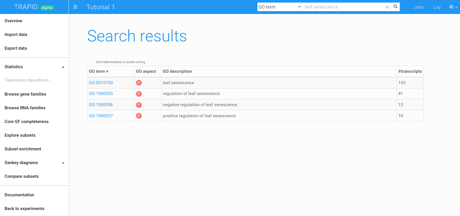
Figure 10: GO term search results for leaf senescence. The GO terms having matching descriptions were retrieved. From here, the associated sequences can rapidly be found.
First, search for leaf senescence GO terms, and look at the transcripts annotated with the leaf senescence (GO:0010150) term by clicking on the GO identifier (Figure 10).
Look at contig04501: this transcript is annotated as 'quasi full length'. Click on its identifier to get to the transcript page. Once there, click the associated gene family identifier, which will take you to its associated gene family page.
From the gene family page, build the multiple sequence alignment (MSA) for this gene family by clicking Create multiple sequence alignment / phylogenetic tree in the toolbox. On the next page, check Generate MSA only to ensure no phylogenetic tree is generated. While it's possible to use MUSCLE instead of MAFFT and to modify the set of input sequences, we will not do so in the tutorial. Click Create MSA/tree to launch the creation of the MSA. Note that if more than 250 genes are selected, it will not be possible to submit the MSA creation job.
After completion, the page will contain a tab with a viewer for the MSA. From the alignment, it can be seen the transcript has indeed a good alignment with most of the other members in the family, although at the N-terminal end there likely is a portion missing (and hence is indeed quasi full length). The other transcript assigned to the family, contig20276, is the opposite: the C-terminal end appears to be missing. Both contigs may therefore represent a single, split transcript.
The Files & extra tab provides a link to download the MSA in .faln format and lists the parameters used to generate it.
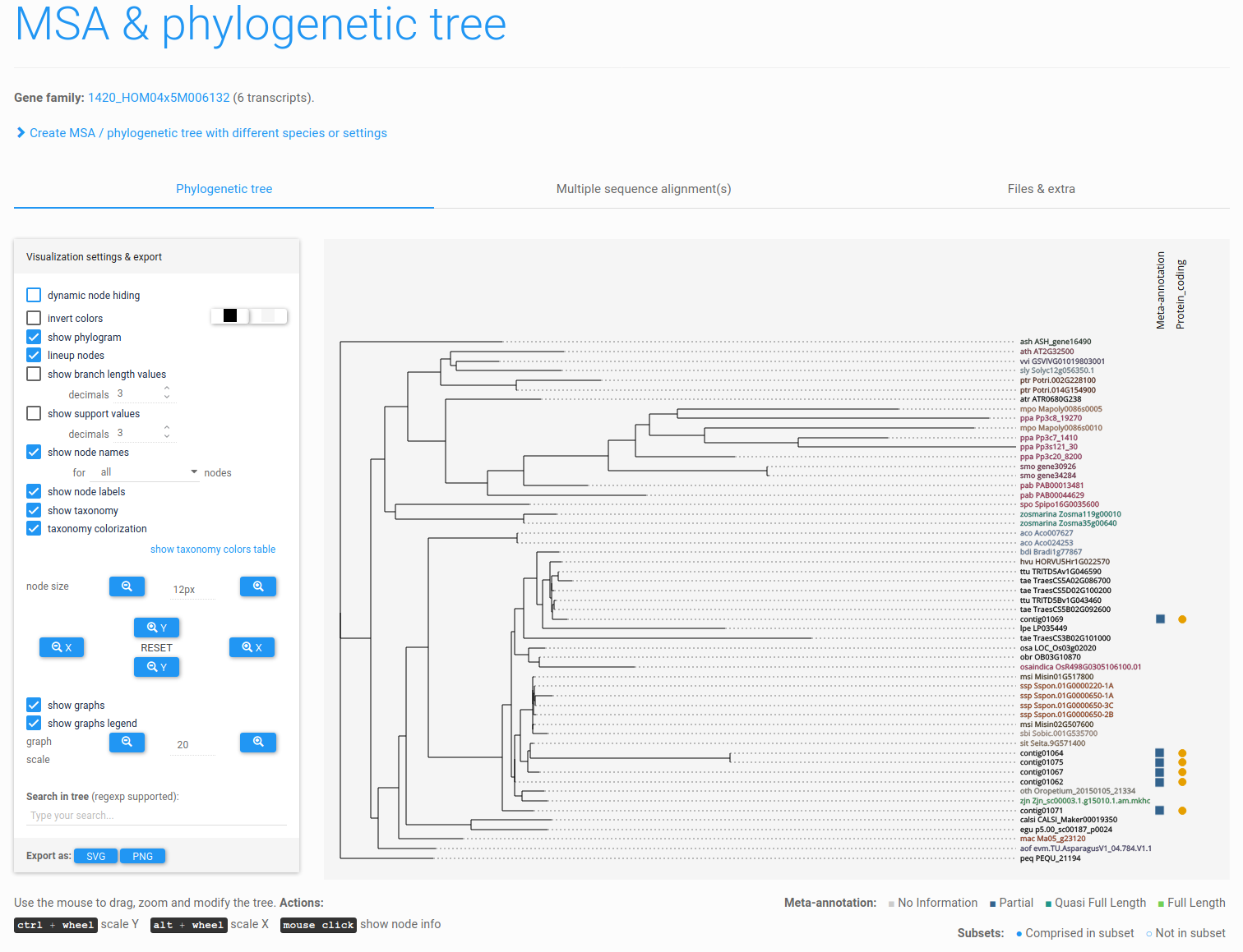
Figure 11: phylogenetic tree. Interactive tree viewer (PhyD3) showing the phylogenetic tree of contig01069 and its homologs. Transcript meta-annotation and subset information are also displayed, depicted next to the transcript identifiers as colored squares and circles, respectively.
Now, search for another transcript: contig01069. Find the gene family page of this transcript and click Create multiple sequence alignment / phylogenetic tree. This time, we will create a phylogenetic tree. In addition to the settings mentioned in the previous part, various phylogenetic tree creation settings can be adjusted: the MSA editing mode, the tree construction algorithm, and tree annotations (extra information about the transcripts displayed next to tree leaves). Feel free to do so (for instance, selecting fewer species from the reference gene family).
Next, click Create MSA / tree. The tree creation job will be launched and an e-mail will be sent upon completion. Once the job has finished, go back to the gene family page and click View or create multiple sequence alignment / phylogenetic tree to view the tree. The page will now contain a tab with an interactive viewer for the generated phylogenetic tree (Figure 11).
In case no tree is displayed or get an error message, very often the selected MSA editing setting is too stringent and should be modified. To check if this is the case, go to the multiple sequence alignment tab, and check the length of the edited alignment: if it is zero amino acids, then the editing was too stringent.
The Files & extra tab provides links to download the tree in PhyloXML and Newick formats and lists the parameters used to generate the phylogenetic tree. In case you want to create a new MSA or tree for the gene family with different settings, simply click the Create MSA / phylogenetic tree […] link on top of the page.
Read more about multiple sequence alignments and phylogenetic trees in the general documentation
Part 4: defining and analyzing subsets (within-transcriptome functional analysis)
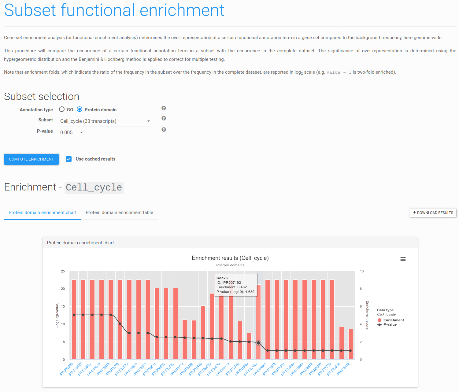
Figure 12: enriched InterPro domains. Overview of InterPro domain enriched within the Cell_cycle subset (maximum corrected p-value 0.005).
Within a TRAPID experiment, transcript subsets can be defined from any arbitrary list of transcript identifiers, for instance transcripts expressed in a specific condition or tissue, and used to perform subsequent within-transcriptome functional analyses. Subsets may either be uploaded as a file or created interactively from the web application. By creating transcript subsets, several new analyses become available, such as comparison of functional annotation between different subsets, or functional enrichment analysis.
In this tutorial, we provide an example set of 33 Cell Cycle transcripts. The list can be downloaded from TRAPID’s FTP. To create a new transcript subset, click Import data (side menu). In the Transcript subset tab, click Browse... to select the downloaded file and enter a name for the subset (e.g. Cell_cycle). Click Import subset to finish.
Transcripts subsets can be inspected and deleted from the Explore subsets page (side menu). To check if the cell cycle set is enriched for specific GO terms or Protein domains, click the Subset enrichment item in the side menu. On the next page, select a type of functional annotation for which to perform the analysis, a transcript subset, and a maximum q-value (corrected p-value) threshold. For this tutorial, we selected InterPro domains, Cell_cycle and 0.005. Click Compute enrichment to launch the analysis.
Figure 12 shows the resulting page displaying for each of the enriched InterPro domains the enrichment fold, significance and a short description. Note that the InterPro domain identifiers are hyperlinks to pages containing more detailed information, and that results may also be explored as a table or downloaded.
It is optionally possible to precompute functional enrichments for all available types of functional annotation, subsets, and q-value thresholds, by clicking the Run functional enrichment button on the experiment overview page.
Read more about subsets/labels and functional enrichment in the general documentation
Tutorial 2: examining gene space completeness
For this second tutorial, we'll continue using the TRAPID experiment created previously. Please make sure that the initial processing has been performed before following this tutorial.
TRAPID enables users to assess and examine the gene space completeness of transcriptomes by checking the presence of core gene families (‘core GFs’), leveraging the GF assignment step of the initial processing.
- Core GFs consist of a set of gene families that are highly conserved in a majority of species within a defined evolutionary lineage.
- Core GF sets can be defined on-the-fly for any clade represented in the selected reference database, making it possible to rapidly examine gene space completeness along an evolutionary gradient.
Read more about the core GF completeness analysis in the general documentation.
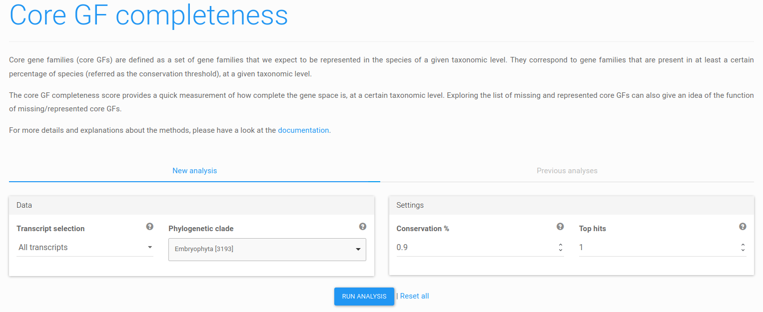
Figure 13: core GF completeness analysis submission form. Any phylogenetic clade represented in the selected reference database may be used for the analysis.
First, click the core GF completeness item of the side menu. The next page, shown in Figure 13, enables submission of core GF completeness jobs (New analysis tab) and exploration of previous analysis results (Previous analysis tab, disabled when no prior analysis was performed). Select a clade for the analysis, and click Run analysis to launch the job. The analysis can take up to a few minutes.
The default value of the conservation threshold parameter is 0.9, meaning that a gene family is considered to be 'core' if it is represented in at least 90% of the species of the selected clade. This threshold does not require complete conservation across all species of the clade and can be adjusted in case more stringent or relaxed conservation requirements are needed.
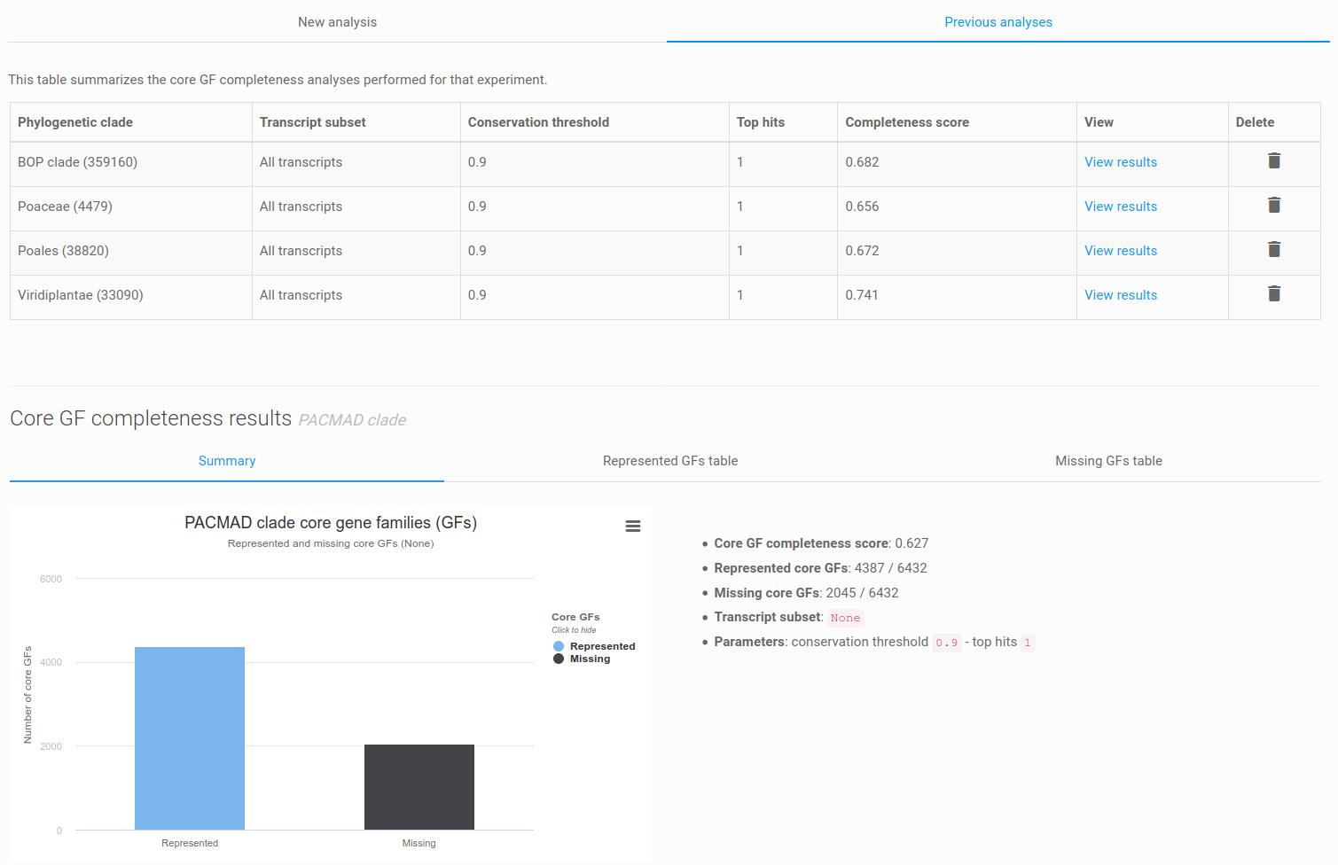
Figure 14: list of previous analyses and core GF completeness result panel. The result panel is organized in three tabs: a summary, the represented GFs table, and the missing GFs table.
After completion of the job, you should now be able to see the result panel (or an error message), composed of three tabs: summary, represented GFs table, and missing GFs table. The summary consists of a bar chart depicting the number of represented and missing core gene families, the completeness score and additional analysis metrics. The represented and missing core gene families, and their associated functional data, can be further investigated using the dedicated tables. It is also possible to export the tables to flat files.
Finally, you can select different clades or settings and re-run the analysis for the same dataset. If you reload the core GF completeness page, the 'previous analyses' tab will be active and list all previous core GF completeness results (Figure 14).